Monte Carlo simulation of CuCl2 in 18.6% aqueous ammonia solution

March 12, 2007 in Computational Chemistry, Journal

The publication below is one of the closest researches to my thesis research. It was carried out by my thesis supervisor in his PhD study. This research emphasized the application of
Monte Carlo simulation in determining structure of Cu(II) in CuCl2 solution. We used similar
Monte Carlo simulation program (Monte Carlo 98). 

Harno Dwi Pranowo^, Austrian-Indonesian Centre for Computational Chemistry (AIC), Department of Chemistry, Faculty of Mathematics and Natural Sciences, Gadjah Mada University, Yogyakarta 55281, Indonesia

Received 11 April 2003.  Available online 23 May 2003.

Abstract

A Monte Carlo simulation was performed for a basic box containing 171 water molecules, 39 ammonia molecules, 5 Cu²⁺, and 10 Cl⁻ ions, corresponding to a 1.3 molal CuCl₂ solution in 18.6% aqueous ammonia, at a temperature of 293.16 K. The results of the Monte Carlo simulation demonstrate that [Cu(NH₃)₄(H₂O)₂]²⁺ is the main species present (49.5%), besides [Cu(NH₃)₂(H₂O)₄]²⁺ (8.0%), [Cu(NH₃)₃(H₂O)₃]²⁺ (14.1%), [Cu(NH₃)₅(H₂O)]²⁺ (28.2%) and small amounts of [Cu(NH₃)₁(H₂O)₅]²⁺ (0.2%). The structure of the solvated ion is discussed in terms of radial distribution functions, coordination number and angular distribution.

Author Keywords: Monte Carlo simulation; Pair and three-body correction functions; Solvation of ion in mixed solvents

 

Article Outline

1. Introduction

2. Details of the calculations

2.1. Pair potential of Cl⁻–NH₃ system

2.2. Three-body potential for Cu²⁺–Cl⁻–NH₃

2.3. Monte Carlo simulation of CuCl₂ in 18.6% aqueous ammonia

3. Results and discussion

3.1. Structural analysis

3.2. Stepwise stability constants of Cu²⁺ amino complex formation

References

 

1. Introduction

The thermodynamics and structural features of mixed solvents are attracted the interest of numerous researchers. Theoretical studies of mixed solvents by Monte Carlo or Molecular Dynamics simulations have been extensively used to obtain information about solvent–solvent interactions such as in methanol–water [1], t-butyl alcohol–water [2], DMSO–water [3], ammonia–water [4], acetone–water [5], hydroxylamine–water [6], and formamide–water [7] mixtures. On the other hand some studies of binary systems with components of different polar nature have also been reported although they represent a small fraction of the simulation work, e.g., papers by Evans about H₂O–CCl₄ mixtures [8] and by Fincham et al. [9 and 10] about CO₂–C₂H₆ mixtures.

The first study of preferential solvation by theoretical means was reported by Narusawa and Nakanishi [11]. The first simulation work on preferential solvation of an ion in a 18.45% mol aqueous ammonia solution was reported in 1988 [12]. Tanabe and Rode studied the solvation of Na⁺ and Kheawsrikul et al. determined the solvent structure around Li⁺ [13] and Mg²⁺ [14] by Monte Carlo method. Kerdcharoen et al. [15] used the combined Quantum Mechanical and Molecular Dynamics (QM/MD) method to study the preferential solvation of Li⁺ in aqueous ammonia solution.

Simulations of aqueous solutions of divalent metal ions based on Monte Carlo method always give overestimated coordination numbers for the first shell, if they are performed with pair potentials only, i.e., neglecting three-body and higher interaction terms, especially when transition metal ions are involved. In order to simulate CuCl₂ in aqueous ammonia solution, we had to include, therefore, five different three-body correction functions.

Nagypal and Debreczeni [16] studied the dynamics of equilibria in aqueous solutions of Cu²⁺–ammonia system by NMR relaxation and pH measurements. The values of the formation constants are slightly increasing for all four complexation steps, but not as drastically as in the relation found in ligand substitution reactions of nickel(II) and cobalt(II) complexes, where the ligand bound to central ion, in general, labilizes the remaining water molecules, thus fastening the further ligand substitution processes. The stepwise stability constants in the Cu²⁺–ammonia system at 25 °C in 2 M NH₄Cl aqueous solution are 2 × 10⁴, 8.4 × 10⁴, 2.9 × 10⁵ and 3 × 10⁶ for [Cu(NH₃)]²⁺, [Cu(NH₃)₂]²⁺, [Cu(NH₃)₃]²⁺ and [Cu(NH₃)₄]²⁺, respectively.

Fabian [17] investigated the kinetics and the mechanism of complex formation of ammonia with Cu²⁺ complexes in 2 mol dm⁻³ of NH₄Cl aqueous solution by temperature-jump relaxation technique. He found that the forward rate constant for the species [Cu(NH₃)]²⁺ is very large (the order is 10⁸) as consequence of the strongly distorted elongated octahedral structure of the metal ion which allows rapid coordination of an entering ligand at the axial position [18].

The simulation of CuCl₂ in ammonia–water mixtures could give us the information about how ammonia, water and chloride ions are preferentially taken by Cu²⁺ into the first and second solvation shell. Energetic and structural properties were evaluated on the basis of Monte Carlo statistical simulation using pair potentials plus Cu²⁺–H₂O–H₂O, Cu²⁺–NH₃–NH₃, Cu²⁺–H₂O–NH₃, Cu²⁺–Cl⁻–H₂O and Cu²⁺–Cl⁻–NH₃ three-body potentials.

2. Details of the calculations

In order to perform the simulation of a system containing CuCl₂ in aqueous ammonia, 10 pair potentials, namely Cu²⁺–Cu²⁺ [19], Cu²⁺–Cl⁻ [20], Cu²⁺–H₂O [21], Cu²⁺–NH₃ [22], Cl⁻–Cl⁻ [23], Cl⁻–H₂O [23], H₂O–H₂O [24], H₂O–NH₃ [4], NH₃–NH₃ [25] and Cl⁻–NH₃ are needed. The first nine pair potentials were available from literature and the Cl⁻–NH₃ pair potential was newly constructed. From the five three-body correction functions Cu²⁺–H₂O–H₂O [21], Cu²⁺–H₂O–NH₃ [26], Cu²⁺–NH₃–NH₃, [22], and Cu²⁺–Cl⁻–H₂O [20] were taken from literature, and the Cu²⁺–Cl⁻–NH₃ three-body potential function was newly constructed.

2.1. Pair potential of Cl⁻–NH₃ system

The Cl⁻–NH₃ pair potential was newly constructed using the same procedure as previously done for Cu²⁺–NH₃ [22]. The basis set proposed by Schäfer et al. [27] was used for chloride and the double-ζ plus polarization (DZP) basis set of Dunning [28] for ammonia. The global minimum of the interaction energy of −11.20 kcal mol⁻¹ was found for the C_3v configuration of the Cl⁻–NH₃ adduct at a Cl⁻–N distance of 3.4 Å.

Fitting of more than 1900 energy points to a functional form was performed by a least-squares method with Levenberg–Marquart algorithm and, testing various potential types in order to describe all electrostatic and van der Waals interactions, resulted in the function
 

(1)

where A_iM, B_iM, and C_iM denote the fitting parameters, r_iM are distances between the ith atom of NH₃ and Cl⁻, q_i are the atomic net charges of the ith atom of NH₃ taken from Mulliken population analysis, and q_M is the charge of Cl⁻. Configurations with energies above +30 kcal mol⁻¹ were excluded and weighting was performed with respect to the absolute and low-lying local energy minima. Identical coefficients were used for equivalent hydrogen atoms. The final parameters of the function are given in Table 1. The standard deviation of the fitted values from SCF data was ± 1.57 kcal mol⁻¹ for the whole region.

Table 1. Final optimized parameters for the interactions of N and H atoms of ammonia with Cl⁻

The atomic net charges are given in a.u., interaction energies and distances in kcal mol⁻¹ and Å, respectively.

2.2. Three-body potential for Cu²⁺–Cl⁻–NH₃

The Cu²⁺–Cl⁻–NH₃ three-body potential function was constructed using the same procedure as previously employed for Cu²⁺–NH₃–NH₃ [22]. For the system consisting of one copper, one chloride and one ammonia molecule, 1200 configurations were generated in the configuration space around the copper ion. The basis sets proposed by Schäfer et al. [27] were used for chloride and copper atoms, and the double-ζ plus polarization (DZP) basis set of Dunning [28] for ammonia.

The three-body interaction energy ΔE_3bd for each configuration was computed by subtracting the two-body interaction E_2b, calculated with the help of the pair potential functions for copper–ammonia, copper–chloride and chloride–ammonia, from the ab initio energies. All three-body data points were fitted to an analytical function to be used as correction for the pair potential. The form of this correction function is
 

(2)

where CL represents the cutoff limit to be used in the simulation, beyond which three-body effects can be neglected. In our case CL was set to 6.0 Å. The parameters of the three-body correction function were obtained by fitting with the Levenberg–Marquart algorithm and the fitted values show a standard deviation of ± 2.1 kcal mol⁻¹.

2.3. Monte Carlo simulation of CuCl₂ in 18.6% aqueous ammonia

The basic box contained 171 water molecules, 39 ammonia molecules, 5 Cu²⁺, and 10 Cl⁻ ions, corresponding to a 1.3 molal CuCl₂ solution in 18.6% aqueous ammonia, at a temperature of 293.16 K. The density for this solution at the specified temperature gives an edge length of 20.85 Å for the elementary box. Periodic boundary condition and cut-off of exponential terms at half of this length were applied. Long-range coulombic interactions were treated by means of Ewald summation. After generating a starting configuration randomly, the system had reached energetic equilibrium after 5 × 10⁶ configurations and additional 3 × 10⁶ configurations were calculated to evaluate radial distribution functions and other structural data.

3. Results and discussion

3.1. Structural analysis

The simulation data were evaluated by combined usage of radial distribution functions, coordination number and angular distribution functions. The characteristic values for the RDFs and average coordination numbers from the simulation are given in Table 2.

Table 2. Characteristic values of the radial distribution functions g_αβ(r) for CuCl₂ in aqueous ammonia; r_M1, r_M2 and r_m1, r_m2 are the distances in Å, where g_αβ(r) are the first and second maximum and the first and second minimum, respectively

n_αβ(m₁) and n_αβ(m₂) are the running integration numbers integrated up to r_m1 and r_m2, respectively.

The Cu–O (Fig. 1) and Cu–N (Fig. 2) RDFs display a peak for the first solvation shell of the ion centered at 2.16 and 2.26 Å, respectively. Since a simulation including no higher than three-body effects cannot account for Jahn–Teller distortion in principle, our values of Cu–O and Cu–N distances appear to be reasonable average of the experimentally determined values between 2.0 and 2.6 Å [29]. Integration up to the first minima of Cu–O and Cu–N RDFs gave on average the coordination number of 4 for ammonia and 2 for water ligands in the first solvation shell. For Cu–H₂O, a second shell peak centered at 3.5 Å is observed, and integrated up to 5.5 Å contains seven water molecules. The average number of ammonia molecules in the second shell between 3.6 and 6.1 Å is 10.3. The Cu–H_W (Fig. 1) and Cu–H_A (Fig. 2) RDFs with the first peak at 2.5–3.6 and 3.7–5.8 Å, respectively, containing 4 and 12 hydrogen atoms, respectively, corresponding to two water and four ammonia molecules. These RDFs indicate also the dipole orientation of ligand molecules in the first solvation shell of copper ion.

Fig. 1. Cu–O/Cu–H_w radial distribution functions and their running integration numbers.

Fig. 2. Cu–N/Cu–H_A radial distribution functions and their running integration numbers.

The Cu–Cl RDF (Fig. 3) clearly shows that no species is formed where chloride binds directly to the Cu²⁺ ion. The double peak between 3.7 and 7 Å, however, shows that solvent separated ion complexes are formed. Integration up to the first local minimum at 5.46 Å yields an average of 3.5 chloride ions, with a “coordination number” of 4 being dominant (Fig. 6).

Fig. 3. Cu–Cl radial distribution function and their running integration number.

Fig. 6. Second shell coordination number distributions of Cu²⁺–Cl.

Coordination number distributions for the first solvation shell of Cu²⁺ were evaluated in order to obtain detailed insight into the composition of the [Cu(NH₃)_n]²⁺ complexes. Fig. 4 and Fig. 5 show the percentage contribution of coordination numbers for water and ammonia ligands, respectively. These figures demonstrate that [Cu(NH₃)₄(H₂O)₂]²⁺ (49.5%) is the main species present, besides [Cu(NH₃)₂(H₂O)₄]²⁺ (8.0%), [Cu(NH₃)₃(H₂O)₃]²⁺ (14.1%), [Cu(NH₃)₅(H₂O)]²⁺ (28.2%) and small amounts of [Cu(NH₃)₁(H₂O)₅]²⁺ (0.2%).

Fig. 4. First and second shell coordination number distributions of Cu²⁺–H₂O.

Fig. 5. First and second shell coordination number distributions of Cu²⁺–NH₃.

The flexibility of ligands in the first solvation shell can be shown in the angle distribution plots for NH₃–Cu–NH₃, H₂O–Cu–NH₃ and H₂O–Cu–H₂O (Fig. 7). The distribution plot of the NH₃–Cu–NH₃ angle shows two peaks centered at 83° and 164° while for NH₃–Cu– H₂O it displays two peaks centered at 92° and 169°. The H₂O–Cu–H₂O angle distribution also displays two peaks centered at 85° and a small peak centered at 161°. From these data, it is clear that – irrespective of eventual further Jahn–Teller distortion not reflected by pair plus three-body potentials – the structure of the [Cu(NH₃)₄(H₂O)₂]²⁺ complex is a distorted octahedron, with the Cu–N distance being longer than the Cu–O distance. The two water molecules never assume a trans position in the octahedron.

Fig. 7. Angular distribution functions for NH₃–Cu–NH₃, NH₃–Cu–H₂O and H₂O–Cu–H₂O in the first solvation shell.

The structure of the first solvation shell of CuCl₂ in 18.6% aqueous ammonia solution is dominated by [Cu(NH₃)₄(H₂O)₂]²⁺ (49.5%), compared to only 14% of [Cu(NH₃)₃(H₂O)₃]²⁺. These values considerably differ from the structure predicted for a single Cu²⁺ ion in 18.6% aqueous ammonia solution, for which only [Cu(NH₃)₃(H₂O)₃]²⁺ is found. One possible explanation is the lack of the long-range interactions for the charged single ion, where long-range corrections had not been performed. However, a comparison of similar single ion-solvent system and related systems containing a balanced amount of cations and anions [30 and 31], for which Ewald corrections have been performed, shows that the differences appear to be marginal at salt concentrations up to 1 molal. Therefore, the difference in species distribution should have other reasons related to the interaction of Cu²⁺ with Cl⁻ ion. Although no [CuCl_n]^(2 − n)+ species is observed in the simulation, Cl⁻ is found at distances corresponding to the second solvation shell, where the anion still interacts considerably with both the cation and adjacent ligand molecules. It is assumed, therefore, that this formation of solvent-separated ion pairs is the main reason for the observed change is species distribution.

3.2. Stepwise stability constants of Cu²⁺ amino complex formation

The thermodynamic stability of a complex can be measured by relating its concentration to the concentration of its components when the system is at equilibrium. From the quantities of [Cu(NH₃)_n]²⁺ species predicted to coexist in the system by the simulation, evaluation of the corresponding consecutive complex formation constants, K_n, is possible. From the coordination number distribution of NH₃ ligands in the first shell of Cu²⁺ (Fig. 5), the percentage occurrence of di-, tri-, tetra- and penta-amino complexes are known and these percentages give the relative concentrations of [Cu(NH₃)]²⁺, [Cu(NH₃)₂]²⁺, [Cu(NH₃)₃]²⁺, [Cu(NH₃)₄]²⁺, and [Cu(NH₃)₅]²⁺ in solution. The concentration of free ligand, [NH₃] is calculated according to the following equation and the stepwise stability constants of Cu²⁺ amino complex formation obtained from the simulation are shown in Table 3
 

[NH3]=[NH3]total−[Cu(NH3)]2+−2[Cu(NH3)2]2+−3[Cu(NH3)3]2+−4[Cu(NH3)4]2+−5[Cu(NH3)5]2+.

(3)

Table 3. Stepwise stability constants of Cu²⁺ amino complex formation obtained from the simulation and experimental

From Table 3, one can see that the stability constants obtained from the first shell composition of complex species of the simulation are smaller than those obtained experimentally, except for K₅, but that the trends of a decrease from K₂ to K₅ and of the great similarity of K₃, K₄ and K₅ are well reflected. One possible explanation for the discrepancies in magnitude is using of concentrations instead of species activities in the simulated system, where the salt concentration is considerably high, namely 1.3 molal. Nagypal and Debreczeni [35] studied the dynamics of equilibria in aqueous solutions of Cu²⁺–ammonia system by NMR relaxation and pH measurements. They measured the stepwise stability constant in Cu²⁺–ammonia system at 25 °C in 2 M NH₄Cl aqueous solution.

 

References

1. S. Okazaki, H. Touhara and K. Nakanishi. J. Chem. Phys. 81 (1984), p. 890. Full Text via CrossRef

2. H. Tanaka, K. Nakanishi and H. Touhara. J. Chem. Phys. 81 (1984), p. 4065. Full Text via CrossRef

3. I.I. Vaisman and M.L. Berkowitz. J. Am. Chem. Soc. 114 (1992), p. 7889. Full Text via CrossRef

4. Y. Tanabe and B.M. Rode. J. Chem. Soc. Faraday Trans. 2 84 (1988), p. 679. Full Text via CrossRef

5. M. Ferrario, M.H. Haughney, I.R. McDonald and M.L. Klein. J. Chem. Phys. 93 (1990), p. 5156. Full Text via CrossRef

6. S. Vizoso, M.G. Heinzle and B.M. Rode. J. Chem. Soc. Faraday Trans. 90 (1994), p. 2337. Full Text via CrossRef

7. Y.P. Puhovski and B.M. Rode. J. Phys. Chem. 99 (1995), p. 1566. Full Text via CrossRef

8. M.W. Evans. J. Chem. Phys. 86 (1987), p. 4096. Full Text via CrossRef

9. D. Fincham, N. Quirke and D.J. Tildesley. J. Chem. Phys. 84 (1986), p. 4535. Full Text via CrossRef

10. D. Fincham, N. Quirke and D.J. Tildesley. J. Chem. Phys. 87 (1987), p. 6117. Full Text via CrossRef

11. H. Narusawa and K. Nakanishi. J. Chem. Phys. 73 (1980), p. 4066. Full Text via CrossRef

12. Y. Tanabe and B.M. Rode. J. Chem. Soc. Faraday Trans. 2 84 (1988), p. 679. Full Text via CrossRef

13. S. Kheawsrikul, S.V. Hannongbua, S.U. Kokpol and B.M. Rode. J. Chem. Soc. Faraday Trans. 2 85 (1989), p. 643. Full Text via CrossRef

14. S. Kheawsrikul, S.V. Hannongbua and B.M. Rode. Z. Naturforsch. 46a (1990), p. 111.

15. T. Kercharoen, K.R. Liedl and B.M. Rode. Chem. Phys. 211 (1996), p. 313.

16. I. Nagypal and F. Debreczeni. Inorg. Chim. Acta 81 (1984), p. 69. Abstract | Abstract + References | PDF (514 K)

17. I. Fabian. J. Chem. Soc. Dalton Trans. (1994), p. 1355. Full Text via CrossRef

18. D.H. Powell, L. Helm and A.E. Merbach. J. Chem. Phys. 95 (1991), p. 9258. Full Text via CrossRef

19. B.M. Rode, S.M. Islam and Y.P. Yongyai. Pure Appl. Chem. 63 (1992), p. 1725.

20. N.R. Texler, S. Holdway, G.W. Neilson and B.M. Rode. J. Chem. Soc., Faraday Trans. 94 (1998), p. 59. Full Text via CrossRef

21. N.R. Texler and B.M. Rode. J. Phys. Chem. 99 (1995), p. 15714. Full Text via CrossRef

22. H.D. Pranowo and B.M. Rode. J. Phys. Chem. A 103 (1999), p. 4298. Full Text via CrossRef

23. P. Bopp, W. Dietz and K. Heinzinger. Z. Naturforsch. A 34 (1979), p. 1424.

24. G. Jancso, K. Heinzinger and P. Bopp. Z. Naturforsch. 34a (1985), p. 1235.

25. S.V. Hannongbua, T. Ishida, E. Sphor and K. Heinzinger. Z. Naturforch. A 43 (1988), p. 572.

26. H.D. Pranowo and B.M. Rode. J. Chem. Phys. 112 (2000), p. 4212. OJPS full text | Full Text via CrossRef

27. A. Schäfer, H. Horn and R. Ahlrichs. J. Chem. Phys. 97 (1992), p. 2571. Full Text via CrossRef

28. T.H. Dunning, Jr.. J. Chem. Phys. 53 (1970), p. 2823. Full Text via CrossRef

29. H. Ohtaki and T. Radnai. Chem. Rev. 93 (1993), p. 1157. Full Text via CrossRef

30. S. Vizoso and B.M. Rode. Chem. Phys. 213 (1996), p. 77. Abstract | Abstract + References | PDF (1313 K)

31. N.R. Texler and B.M. Rode. Chem. Phys. 222 (1997), p. 281. Abstract | Abstract + References | PDF (426 K)

32. J. Inczedy, Analytical Applications of Complex Equilibria. , Ellis Horwood limited, England (1976).

33. F. Seel, Grundlagen der Analytischen Chemie. (fourth ed.),, Verlag Chemie, Weinheim (1965).

34. T.R. Blackburn, Equilibrium, a Chemistry of Solutions. , Holt, Reinhart and Winston, Inc., New York (1969).

35. I. Nagypal and F. Debreczeni. Inorg. Chim. Acta 81 (1984), p. 69. Abstract | Abstract + References | PDF (514 K)

 

Corresponding author. Tel.: +62-274-545188; fax: +62-274-545188

Chemical Physics
Volume 291, Issue 2 , 15 June 2003, Pages 153-159

Mefloquine Antimalarial Drugs

March 8, 2007 in Drugs Design, My Research Expansion

Mefloquine is an orally administered antimalarial drug used as a prophylaxis against and treatment for malaria. It also goes by the trade name Lariam® (manufactured by Roche Pharmaceuticals) and chemical name mefloquine hydrochloride (formulated with HCl). Mefloquine was developed in the 1970s at the Walter Reed Army Institute of Research in the U.S. as a chemical synthetic similar to quinine.

Uses

Mefloquine is used to prevent malaria (malaria prophylaxis) and also in the treatment of chloroquine-resistant falciparum malaria. As mefloquine resistance spreads, mefloquine has started to lose its efficacy. Mefloquine is the drug of choice to treat malaria (though not necessarily to prevent malaria) caused by chloroquine-resistant Plasmodium vivax.

Advice to travelers

Mefloquine is one of the antimalarial drugs which the August 2005 issue of the CDC Travel Health Yellow Sheet advises travelers in areas with malaria risk — Africa, South America, the Indian subcontinent, Asia, and the South Pacific — to take. Other medicines with less risk of severe side-effects and which are equally effective for malaria prevention are Malarone and doxycycline.There are virulent strains of malaria that are resistant to one or more anti-malarial drugs; for example, there are mefloquine-resistant strains in Thailand, Cambodia and Myanmar. Travelers are advised to compare current recommendations before selecting an antimalarial drug as the occurrence of drug-resistant strains changes.The CDC, the UK Guidelines for Malaria Prevention, and the WHO provide up-to-date recommendations for specific countries.The drug is taken once a week starting at least one week prior to entry into malaria endemic areas and continued for 4 weeks after leaving. Owing to the risk of neuropsychiatric disturbance, particularly disruption of sleep, UK advice is for people who have not previously used Mefloquine to start 3 weeks prior to departure; adverse effects usually manifest within one or two weeks, and so there would remain sufficient time to switch to an alternative drug.

Side-effects

Mefloquine may have severe and permanent adverse side-effects. It is known to cause severe depression, anxiety, paranoia, nightmares, insomnia, seizures, peripheral motor-sensory neuropathy, vestibular (balance) damage and central nervous system problems. For a complete list of adverse physical and psychological effects — including suicidal ideation — see the most recent product information. Central nervous system events occur in up to 25% of people taking Lariam, such as dizziness, headache, insomnia, and vivid dreams. In 2002 the word “suicide” was added to the official product label, though proof of causation has not been established. Since 2003, the Food and Drug Administration (FDA) has required that patients be screened before mefloquine is prescribed. The latest Consumer Medication Guide to Lariam has more complete information.In the 1990s there were reports in the media that the drug may have played a role in the Somalia Affair, which involved the torture and murder of a Somali citizen whilst in the custody of Canadian peacekeeping troops. There has been similar controversy since three murder-suicides involving Special Forces soldiers at Fort Bragg, N.C., in the summer of 2002. To date more than 19 cases of vestibular damage following the use of mefloquine have been diagnosed by military physicians. The same damage has been diagnosed among business travelers and tourists.

Neurological activity

In 2004, researchers found that mefloquine in adult mice blocks connexins called Cx36 and Cx50. Cx36 is found in the brain and Cx50 is located in the eye lens. Connexins in the brain are believed to play a role in movement, vision and memory.

Chirality and its implications

Mefloquine is a chiral molecule with two asymmetric carbon centres, which means it has four different diastereomers. The drug is currently manufactured and sold as a racemate of the (+/-) R*,S* enantiomers by Hoffman-LaRoche, a Swiss pharmaceutical company. According to some research, the (+) enantiomer is more effective in treating malaria, and the (-) enantiomer specifically binds to adenosine receptors in the central nervous system, which may explain some of its psychotropic effects. Some believe that it is irresponsible for a pharmaceutical company to sell mefloquine as a racemic mixture. It is not known whether mefloquine goes through stereoisomeric switching in vivo.

Popular culture references

• Mefloquine was featured in an episode, “Goliath” of the television series Law and Order: SVU as “Quinium”.
• Anthony Frosh, in The Frosh Report, records what he claims is his Mefloquine produced dream diary^.

External links

• Manufacturer’s information page
• Lariam Action USA, Clearinghouse for information on mefloquine news, research, toxicity
• 2004 UPI story about military suicides
• Senator Feinstein Urges Rumsfeld to Complete Lariam Study.
• Discussion of Lariam side-effects at PeaceCorpsOnline.org

References

1. Maguire JD, Krisin, Marwoto H, Richie TL, Fryauff DJ, Baird JK (2006). “Mefloquine is highly efficacious against chloroquine-resistant Plasmodium vivax malaria and Plasmodium falciparum malaria in
   Papua, Indonesia”. Clin Infect Dis 42 (8): 1067–72. 
2. Jha S, Kumar R, Kumar R. (2006). “Mefloquine toxicity presenting with polyneuropathy—a report of two cases in
   India”. Trans R Soc Trop Med Hyg 100 (6): 594–96. DOI:10.1016/j.trstmh.2005.08.006. 
3. Somalia and Mefloquine
4. Scott J. Cruikshank, Matthew Hopperstad, Meg Younger, Barry W. Connors, David C. Spray, Miduturu Srinivas, “Potent block of Cx36 and Cx50 gap junction channels by mefloquine,” Proceedings of the National Academy of Sciences of the United States of America, 101(33), 2004 August 17.
5. Mark Benjamin. Ripped from my headlines!. salon.com
6. Frosh Report discussing dream-altering effects of mefloquine

• Phillips-Howard, P. A., and F. O. ter Kuile. 1995. CNS adverse events associated with antimalarial agents: fact or fiction? Drug Saf. a370-383.

Antimalarial drugs (P01B) edit
Aminoquinolines:	Amodiaquine, Chloroquine, Hydroxychloroquine, Pamaquine, Primaquine
Biguanides:	Proguanil, Cycloguanil embolate
Methanolquinolines:	Mefloquine, Quinine
Diaminopyridines:	Pyrimethamine
Artemisinin derivatives:	Artemisinin, Artemether, Artesunate, Artemotil, Artenimol
Others:	Halofantrine, Lumefantrine

Source: Wikipedia

Another Application of Monte Carlo Simulation

March 8, 2007 in Computational Chemistry, Journal

Monte carlo simulations of the solution structure of simple alcohols

in water-acetonitrile mixtures.

• Nagy PI,
• Erhardt PW.

Center for Drug Design and Development, College of Pharmacy, The University of Toledo, Toledo, OH 43606-3390, USA. pnagy@utnet.utoledo.edu

Monte Carlo simulations have been performed to explore the solution structure of ethyl, isopropyl, isobutyl, and tertiary butyl alcohols in pure water, pure acetonitrile, and different mixtures of the two solvents. The explicit solvent studies in NpT ensembles at T = 298 K illustrate that the solute “discriminates” the solvent’s components and that the composition of the first solvation shell differs from that of the bulk solution. Since the polarizable continuum dielectric method (PCM) does not presently model the solvation of molecules with both polar and apolar sites in mixed protic solvents, we suggest a direction for further program development wherein a continuum dielectric method would accept more than one solvent and the solute sites would be solvated by user-defined solvent components. The prevailing solvation model will be determined upon the lowest free energy calculated for a particular solvation pattern of the solute having a specific conformational/tautomeric state. Characterization of equilibrium hydrogen-bond formation becomes a complicated problem that depends on the chemical properties of the solute and its conformation, as well as upon the varying nature of the first solvation shell. For example, while the number of hydrogen bonds to secondary and tertiary alcohol solutes are nearly constant in pure water and in water-acetonitrile mixtures with at least 50% water content, the number of hydrogen bonds to primary alcohols gradually decreases for most of their conformations when acetonitrile content is increased. Nonetheless, the calculations indicate that O-H…O(water) hydrogen bonds are still possible in a small fraction of the arrangements for the solution models with water content of 30% or less. The isopentene solute does not form any observable hydrogen bonds, despite having an electron-rich, double-bond site.

PMID: 16851638 [PubMed – in process]

1: J Phys Chem B Condens Matter Mater Surf Interfaces Biophys. 2005 Mar 31;109(12):5855-72

Monte Carlo Method

March 7, 2007 in Computational Chemistry

A Monte Carlo algorithm is often a numerical
Monte Carlo method used to find solutions to mathematical problems (which may have many variables) that cannot easily be solved, for example, by integral calculus, or other numerical methods. For many types of problems, its efficiency relative to other numerical methods increases as the dimension of the problem increases. Or it may be a method for solving other mathematical problems that relies on (pseudo-)random numbers

Applications

Monte Carlo simulation methods are especially useful in studying systems with a large number of coupled degrees of freedom, such as liquids, disordered materials, strongly coupled solids, and cellular structures (see cellular Potts model). More broadly,
Monte Carlo methods are useful for modeling phenomena with significant uncertainty in inputs, such as the calculation of risk in business. A classic use is for the evaluation of definite integrals, particularly multidimensional integrals with complicated boundary conditions.Monte Carlo methods are very important in computational physics, physical chemistry, and related applied fields, and have diverse applications from complicated quantum chromodynamics calculations to designing heat shields and aerodynamic forms.Monte Carlo methods have also proven efficient in solving coupled integral differential equations of radiation fields and energy transport, and thus these methods have been used in global illumination computations which produce photorealistic images of virtual 3D models, with applications in video games, architecture, design, computer generated films, special effects in cinema, business, economics and other fields.
Monte Carlo methods are useful in many areas of computational mathematics, where a lucky choice can find the correct result. A classic example is Rabin’s algorithm for primality testing: for any n which is not prime, a random x has at least a 75% chance of proving that n is not prime. Hence, if n is not prime, but x says that it might be, we have observed at most a 1-in-4 event. If 10 different random x say that n is probably prime when it is not, we have observed a one-in-a-million event. In general a Monte Carlo algorithm of this kind produces one correct answer with a guarantee n is composite, and x proves it so, but another one without, but with a guarantee of not getting this answer when it is wrong too often – in this case at most 25% of the time. See also Las Vegas algorithm for a related, but different, idea.

Application in Chemistry

Areas of application include:

• In simulated annealing for protein structure prediction
• In semiconductor device research, to model the transport of current carriers
• Environmental science, dealing with contaminant behaviour
• Monte Carlo method in statistical physics; in particular, Monte Carlo molecular modeling as an alternative for computational molecular dynamics.
• In Physical chemistry, particularly for simulations involving atomic clusters
• Modelling the movement of impurity atoms (or ions) in plasmas in existing and tokamaks (e.g.: DIVIMP).
• In experimental particle physics, for designing detectors, understanding their behaviour and comparing experimental data to theory
• Nuclear and particle physics codes using the
  Monte Carlo method:
  • GEANT – CERN‘s
    Monte Carlo for high-energy particles physics
  • MCNP(X) – LANL’s radiation transport codes
  • EGS – Stanford‘s simulation code for coupled transport of electrons and photons
  • PEREGRINE – LLNL’s
    Monte Carlo tool for radiation therapy dose calculations
  • Modelling of foam and cellular structures
  • Modeling of tissue morphogenesis

Other Methods Employing
Monte Carlo

• Assorted random models, e.g. self-organised criticality
• Direct simulation Monte Carlo
• Dynamic Monte Carlo method
• Kinetic Monte Carlo
• Quantum Monte Carlo
• Quasi-Monte Carlo method using low-discrepancy sequences and self avoiding walks
• Semiconductor charge transport and the like
• Electron microscopy beam-sample interactions
• Stochastic Optimization
• Cellular Potts model
• Markov chain Monte Carlo

Integration methods

• Direct sampling methods
  • Importance sampling
  • Stratified sampling
  • Recursive stratified sampling
  • VEGAS algorithm
• Random walk Monte Carlo including Markov chains
  • Metropolis-Hastings algorithm
• Gibbs sampling

Optimization

Another powerful and very popular application for random numbers in numerical simulation is in numerical optimization. These problems use functions of some often large-dimensional vector that are to be minimized (or maximized). Many problems can be phrased in this way: for example a computer chess program could be seen as trying to find the optimal set of, say, 10 moves which produces the best evaluation function at the end. The traveling salesman problem is another optimization problem. There are also applications to engineering design, such as multidisciplinary design optimization.Most
Monte Carlo optimization methods are based on random walks. Essentially, the program will move around a marker in multi-dimensional space, tending to move in directions which lead to a lower function, but sometimes moving against the gradient.

Optimization methods

• Evolution strategy
• Genetic algorithms
• Parallel tempering
• Simulated annealing
• Stochastic tunneling

Inverse problems

Probabilistic formulation of inverse problems leads to the definition of a probability distribution in the model space. This probability distribution combines a priori information with new information obtained by measuring some observable parameters (data). As, in the general case, the theory linking data with model parameters is nonlinear, the a posteriori probability in the model space may not be easy to describe (it may be multimodal, some moments may not be defined, etc.).When analyzing an inverse problem, obtaining a maximum likelihood model is usually not sufficient, as we normally also wish to have information on the resolution power of the data. In the general case we may have a large number of model parameters, and an inspection of the marginal probability densities of interest may be impractical, or even useless. But it is possible to pseudorandomly generate a large collection of models according to the posterior probability distribution and to analyze and display the models in such a way that information on the relative likelihoods of model properties is conveyed to the spectator. This can be accomplished by means of an efficient
Monte Carlo method, even in cases where no explicit formula for the a priori distribution is available.The best-known importance sampling method, the Metropolis algorithm, can be generalized, and this gives a method that allows analysis of (possibly highly nonlinear) inverse problems with complex a priori information and data with an arbitrary noise distribution. For details, see Mosegaard and Tarantola (1995) [1] , or Tarantola (2005) [2] .

Monte Carlo And Random Numbers

Interestingly, Monte Carlo simulation methods do not generally require truly random numbers to be useful – for other applications, such as primality testing, unpredictability is vital (see
Davenport (1995) [3]). Many of the most useful techniques use deterministic, pseudo-random sequences, making it easy to test and re-run simulations. The only quality usually necessary to make good simulations is for the pseudo-random sequence to appear “random enough” in a certain sense.What this means depends on the application, but typically they should pass a series of statistical tests. Testing that the numbers are uniformly distributed or follow another desired distribution when a large enough number of elements of the sequence are considered is one of the simplest, and most common ones.

History

Monte Carlo methods were originally practiced under more generic names such as “statistical sampling”. The “Monte Carlo” designation, popularized by early pioneers in the field (including Stanislaw Marcin Ulam, Enrico Fermi, John von Neumann and Nicholas Metropolis), is a reference to the famous casino in Monaco. Its use of randomness and the repetitive nature of the process are analogous to the activities conducted at a casino. Stanislaw Marcin Ulam tells in his autobiography Adventures of a Mathematician that the method was named in honor of his uncle, who was a gambler, at the suggestion of Metropolis.“Random” methods of computation and experimentation (generally considered forms of stochastic simulation) can be arguably traced back to the earliest pioneers of probability theory (see, e.g., Buffon’s needle, and the work on small samples by William Gosset), but are more specifically traced to the pre-electronic computing era. The general difference usually described about a
Monte Carlo form of simulation is that it systematically “inverts” the typical mode of simulation, treating deterministic problems by first finding a probabilistic analog. Previous methods of simulation and statistical sampling generally did the opposite: using simulation to test a previously understood deterministic problem. Though examples of an “inverted” approach do exist historically, they were not considered a general method until the popularity of the
Monte Carlo method spread.Perhaps the most famous early use was by Enrico Fermi in 1930, when he used a random method to calculate the properties of the newly-discovered neutron. Monte Carlo methods were central to the simulations required for the Manhattan Project, though were strongly limited by the computational tools at the time. However, it was only after electronic computers were first built (from 1945 on) that
Monte Carlo methods began to be studied in depth. In the 1950s they were used at Los Alamos for early work relating to the development of the hydrogen bomb, and became popularized in the fields of physics, physical chemistry, and operations research. The Rand Corporation and the U.S. Air Force were two of the major organizations responsible for funding and disseminating information on
Monte Carlo methods during this time, and they began to find a wide application in many different fields.Uses of
Monte Carlo methods require large amounts of random numbers, and it was their use that spurred the development of pseudorandom number generators, which were far quicker to use than the tables of random numbers which had been previously used for statistical sampling.

See also

• Markov chain
• Monte Carlo integration
• Quasi-Monte Carlo method
• Randomness
• Las Vegas algorithm
• Random number generator

References

• Bernd A. Berg, Markov Chain
  Monte Carlo Simulations and Their Statistical Analysis (With Web-Based Fortran Code), World Scientific 2004, ISBN 981-238-935-0.
• Arnaud Doucet, Nando de Freitas and Neil Gordon, Sequential
  Monte Carlo methods in practice, 2001, ISBN 0-387-95146-6.
• P. Kevin MacKeown, Stochastic Simulation in Physics, 1997, ISBN 981-3083-26-3
• Harvey Gould & Jan Tobochnik, An Introduction to Computer Simulation Methods, Part 2, Applications to Physical Systems, 1988, ISBN 0-201-16504-X
• C.P. Robert and G. Casella. “Monte Carlo Statistical Methods” (second edition).
  New York: Springer-Verlag, 2004, ISBN 0-387-21239-6
• Mosegaard, Klaus., and Tarantola, Albert, 1995.
  Monte Carlo sampling of solutions to inverse problems. J. Geophys. Res., 100, B7, 12431-12447.
• Tarantola, Albert, Inverse Problem Theory (free PDF version), Society for Industrial and Applied Mathematics, 2005. ISBN 0-89871-572-5
• Nicholas Metropolis, Arianna W. Rosenbluth, Marshall N. Rosenbluth, Augusta H. Teller and Edward Teller, “Equation of State Calculations by Fast Computing Machines”, Journal of Chemical Physics, volume 21, p. 1087 (1953) (DOI: 10.1063/1.1699114)
• N. Metropolis and S. Ulam, “The Monte Carlo Method”, Journal of the American Statistical Association, volume 44, p. 335 (1949)
• Fishman, G.S., (1995) Monte Carlo: Concepts, Algorithms, and Applicatioins, Springer Verlag,
  New York.

External links

• Overview and reference list, Mathworld
• Introduction to Monte Carlo Methods, Computational Science Education Project
• Overview of formula’s used Monte Carlo simulation, the Quant Equation Archive, at sitmo.com
• Monte Carlo Method, riskglossary.com
• The Basics of Monte Carlo Simulations, University of Nebraska-Lincoln
• Introduction to Monte Carlo simulation (for Excel), Wayne L. Winston
• Monte Carlo Simulation, Prof. Don M. Chance
• Monte Carlo Methods – Overview and Concept, brighton-webs.co.uk
• Molecular Monte Carlo Intro, Cooper Union
• Monte Carlo techniques applied to finance, Simon Leger
• MonteCarlo Simulation in Finance, global-derivatives.com
• Approximation of π with the Monte Carlo Method
• Risk Analysis in Investment Appraisal, The Application of
  Monte Carlo Methodology in Project Appraisal, Savvakis C. Savvides
• Primality Testing RevisitedProc. ISSAC 1992, James H. Davenport
• Example of Calculating Pi using the Monte Carlo method, C++
• Probabilistic Assessment of Structures using the Monte Carlo method, Wikiuniversity paper for students of Structural Engineering

[edit] Software

• w3mcsim – Online Monte Carlo Simulation
• The BUGS project (including WinBUGS and OpenBUGS)
• Monte Carlo Simulation Software for Excel by Master Solutions
• Monte Carlo Simulation Tool for Excel by Decisioneering
• Monte Carlo Simulation Tool for Excel by Palisade
• Monte Carlo Simulation Tool for Excel by Lumenaut
• Monte Carlo Simulation for Environmental, Business, and Engineered Systems
• Monte Carlo GridServer DataSynapse Grid Computing Software for
  Monte Carlo

Retrieved from “http://en.wikipedia.org/wiki/Monte_Carlo_method“ 

7 Tools In Quality Control

March 7, 2007 in Industrial Work

Production environments that utilize modern quality control methods are dependant upon statistical literacy. The tools used therein are called the 7 quality control tools.

1. Checksheet

The function of a checksheet is to present information in an efficient, graphical format. This may be accomplished with a simple listing of items. However, the utility of the checksheet may be significantly enhanced, in some instances, by incorporating a depiction of the system under analysis into the form.

2. Pareto Chart

Pareto charts are extremely useful because they can be used to identify those factors that have the greatest cumulative effect on the system, and thus screen out the less significant factors in an analysis. Ideally, this allows the user to focus attention on a few important factors in a process.

They are created by plotting the cumulative frequencies of the relative frequency data (event count data), in decending order. When this is done, the most essential factors for the analysis are graphically apparent, and in an orderly format.

3. Flowchart

Flowcharts are pictorial representations of a process. By breaking the process down into its constituent steps, flowcharts can be useful in identifying where errors are likely to be found in the system.

4. Cause & effect Diagram

This diagram, also called an Ishikawa diagram (or fish bone diagram), is used to associate multiple possible causes with a single effect. Thus, given a particular effect, the diagram is constructed to identify and organize possible causes for it.

The primary branch represents the effect (the quality characteristic that is intended to be improved and controlled) and is typically labelled on the right side of the diagram. Each major branch of the diagram corresponds to a major cause (or class of causes) that directly relates to the effect. Minor branches correspond to more detailed causal factors. This type of diagram is useful in any analysis, as it illustrates the relationship between cause and effect in a rational manner.

 5. Histogram

Histograms provide a simple, graphical view of accumulated data, including its dispersion and central tendency. In addition to the ease with which they can be constructed, histograms provide the easiest way to evaluate the distribution of data.

 

 6. Scatter diagram

Scatter diagrams are graphical tools that attempt to depict the influence that one variable has on another. A common diagram of this type usually displays points representing the observed value of one variable corresponding to the value of another variable.

7. Control Chart

The control chart is the fundamental tool of statistical process control, as it indicates the range of variability that is built into a system (known as common cause variation). Thus, it helps determine whether or not a process is operating consistently or if a special cause has occurred to change the process mean or variance.

The bounds of the control chart are marked by upper and lower control limits that are calculated by applying statistical formulas to data from the process. Data points that fall outside these bounds represent variations due to special causes, which can typically be found and eliminated. On the other hand, improvements in common cause variation require fundamental changes in the process.

Source: http://deming.eng.clemson.edu/

Definition of Molecular Dynamics

February 12, 2007 in Computational Chemistry, My Research Expansion
Tags: Computational Chemistry, molecular dynamics, molecular simulation

 

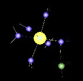
The picture above was about molecular dynamics simulation of  Mg(II) ion solvated in 53 water molecules.

Molecular Dynamics (MD) is a form of computer simulation where atoms and molecules are allowed to interact for a period of time under known laws of physics. Because in general molecular systems consist of a large number of particles, it is impossible to find the properties of such complex systems analytically. MD simulation circumvents this problem by using numerical methods. It represents an interface between laboratory experiments and theory and can be understood as a virtual experiment.

Even though we know matter consists of interacting particles in motion at least since Boltzmann in the 19th Century, many still think of molecules as rigid museum models. Richard Feynman said in 1963 that “everything that living things do can be understood in terms of the jiggling and wiggling of atoms.” One of MD’s key contributions is creating awareness that molecules like proteins and DNA are machines in motion. MD probes the relationship between molecular structure, movement and function.

Molecular dynamics is a multidisciplinary field. Its laws and theories stem from mathematics, physics and chemistry. MD employs algorithms from computer science and information theory. It was originally conceived within theoretical physics in the 1950’s, but is applied today mostly in materials science and biomolecules.

Before it became possible to simulate molecular dynamics with computers, some undertook the hard work of trying it with physical models such as macroscopic spheres. The idea was to arrange them to replicate the properties of a liquid. Here’s a quote from J.D. Bernal from 1962: “… I took a number of rubber balls and stuck them together with rods of a selection of different lengths ranging from 2.75 to 4 inch. I tried to do this in the first place as casually as possible, working in my own office, being interrupted every five minutes or so and not remembering what I had done before the interruption.” ^[3] Fortunately, now computers keep track of bonds during a simulation.

Molecular dynamics is a specialized discipline of molecular modeling and computer simulation based on statistical mechanics; the main justification of the MD method is that statistical ensemble averages are equal to time averages of the system, known as the ergodic hypothesis. MD has also been termed “statistical mechanics by numbers” and “Laplace’s vision of Newtonian mechanics” of predicting the future by animating nature’s forces^{[citation needed]} and allowing the direct visualization of molecular motion on an atomic scale. However, long MD simulations are mathematically ill-conditioned, generating cumulative errors in numerical integration that can be minimized with proper selection of algorithms and parameters, but cannot be eliminated entirely. Further, current potential functions are in many cases insufficiently accurate for reproducing the dynamics of molecular systems. Nevertheless, molecular dynamics techniques allow detailed time and space resolution into representative behavior in phase space.

Source: Wikipedia

MOLVISION, New Visualization of Chemical System

February 10, 2007 in Computational Chemistry, Further thesis study
Tags: Computational Chemistry, monte carlo simulation

The movie above is about:

 Ni(II) – NH3 Complexes in Water Dynamics  (QM/MM-MD Simulation)

with increasing number of heteroligands (di-, tri-, and tetramine complexes) the exchange dynamics for water ligands are accelerated and become observable in the picosecond range

**Molvision is a new flexible tool to visualize chemical systems, from simple molecules to large biopolymers and dynamics of liquids and multi-component solutions. The user can define all atom and bond characteristics according to needs and taste, via the comfortable graphic interface, and every visualisation can be converted to high-quality pictures or video clips by mouse click. Radial distribution functions can be evaluated “on the fly” for any selected pair of atom types.

Basic Definition of Computational Chemistry

February 9, 2007 in Computational Chemistry
Tags: Computational Chemistry, theoretical chemistry

Computational Chemistry is a branch of chemistry that use the product of theoretical chemistry that is translated into computational program to calculate molecular properties and its changes and also to perform simulation to macromolecules system (such as proteins, or system with a huge number of molecules such as gasses, liquid and liquid crystal) and apply the program to the real chemical system. The examples of molecular properties that are calculated are structures (the positions of atoms), energy and deviation energy, charges, dipole moments, reactivity, wave frequency, and other spectroscopy measurements. Simulation to macromolecules (such proteins, and nucleic acid) and large system can include the study of molecule conformation and its change (for example denaturising process of protein), phase change, and also prediction of macroscopic properties (such typical heat) based on properties in atomic level and molecules. The term of computational chemistry sometimes also used for interdisciplinary studies between computer science and chemistry. The term of theoretical chemistry can be defined as mathematics description for chemistry, while computational chemistry usually used when mathematics method are developed well to be used in computer program. Please note that the word ‘exact’ or ‘perfect’ will not appear here because is very little of chemistry aspects can be calculated exactly. Almost all chemical aspects can be described in qualitative computational scheme or qualitative equation.Molecules consist of core and electrons; therefore it needs quantum mechanics method.

Computational chemist usually try to solve Schrödinger equation non relativistic with the addition of relativistic correlation even though some development has been done to solve Schrödinger equation not only in the form of time dependent but also non- time dependent, suited with the problem observed. But it its practical term, it is impossible except for the system that is very small. Therefore, a big number of approximation methods were developed to reach best compromise between the accuracy of calculation and computational cost.In theoretical chemistry, chemist and physicist are together in developing algorithms and computer program to make it possible for prediction of atomic and molecular properties and or reaction path for chemical reaction and also the simulation of macromolecular system.

Computational chemists mostly only use the computer program and available methodology and apply for certain chemistry problems. In the most part of time that they use, computational chemist can also involved in the new algorithms development also the determination of chemical theory that is suitable so that the most efficient and accurate computational process.There are some approximations that can be used:

1.  Computational study can be done to determine the starting point for the synthesis in laboratory.
2. Computational study can be used to explore reaction mechanism and explain the observation of reaction in laboratory.
3. Computational study can be done to understand the property and change of macroscopic system through simulation that based on interaction law that are in the system.

There are some main fields in this topic, i.e.: 

•  Presentation of atomic and molecular computation
•  Approximation in the storing and search of chemical species (chemical basis data)
• Approximation and determination of pattern and relationship between chemical structures and their properties (QSPR, QSAR).
• Structural elucidation theoretically based on simulation of forces.
• Computational approximation to help efficient of material synthesis.
• Computational approximation to design molecules that are interacted by special paths, especially in drugs design.
• Simulation of phases transition
• Simulation of materials such as polymer, metal, and crystal (include liquid crystal)

Program that can be used in computational chemistry based on various chemical quantum methods that solve Schrödinger equation for molecules and also classical physics approximation to simulate huge system.Chemical quantum methods that do not include empirical parameters and semi empirical parameters in their equations are so-called ab initio. Abs Initio methods type that are popular are: Hartree-Fock, Perturbation theory, Møller-Plesset, configuration interaction, coupled cluster, reducted matrix density and density function theory. Molecular Computation: Molecular properties such energy, structure, dipole momen, polarity or hyperpolarizability are some measurements that can be calculated by calculation. In molecular calculation there are some techniques to calculate molecular properties: molecular mechanics, density function theory or electron structure theory.Software packages:The number of software that provide many chemical quantum method. Some of them that are largely in use are:

• Gaussian
• Gamess
• Q-Chem
• NWChem
• ACES
• Molpro
• Dalton
• Spartan
• Psi
• PLATO (Package for Linear Combination of Atomic Orbitals)

See also:

• ·         Quantum Mechanics
• ·         Molecular Mechanics
• ·         Statistical mechanics
• ·         Density Functional Theory
• ·         Force Fields
• ·         Molecular Modelling
• ·         Molecular Dynamics
• ·         Monte Carlo Methods
• ·         QSPR
• ·         Important publications in computational chemistry
• ·         Bioinformatics 

Source: ·          Computational Chemistry from Wikipedia in English. ·          Christopher J. Cramer, Essentials of Computational Chemistry: Theories and Models, 2nd edition, 2004. ·          David C. Young, Computational Chemistry, 2001 ·      

Basics of Wet Analysis Technique: Buret

February 9, 2007 in Analytical Chemistry

A buret is used to deliver solution in precisely-measured, variable volumes. Burets are used primarily for titration, to deliver one reactant until the precise end point of the reaction is reached.

To fill a buret, close the stopcock at the bottom and use a funnel. You may need to lift up on the funnel slightly, to allow the solution to flow in freely.

You can also fill a buret using a disposable transfer pipet. This works better than a funnel for the small, 10 mL burets. Be sure the transfer pipet is dry or conditioned with the titrant, so the concentration of solution will not be changed.Before titrating, condition the buret with titrant solution and check that the buret is flowing freely. To condition a piece of glassware, rinse it so that all surfaces are coated with solution, then drain. Conditioning two or three times will insure that the concentration of titrant is not changed by a stray drop of water.

 

Check the tip of the buret for an air bubble. To remove an air bubble, whack the side of the buret tip while solution is flowing. If an air bubble is present during a titration, volume readings may be in error.

 

 Rinse the tip of the buret with water from a wash bottle and dry it carefully. After a minute, check for solution on the tip to see if your buret is leaking. The tip should be clean and dry before you take an initial volume reading.

 

 

 

When your buret is conditioned and filled, with no air bubbles or leaks, take an initial volume reading. A buret reading card with a black rectangle can help you to take a more accurate reading. Read the bottom of the meniscus. Be sure your eye is at the level of meniscus, not above or below. Reading from an angle, rather than straight on, results in a parallax error. 

Deliver solution to the titration flask by turning the stopcock. The solution should be delivered quickly until a couple of mL from the endpoint.

The endpoint should be approached slowly, a drop at a time. Use a wash bottle to rinse the tip of the buret and the sides of the flask. Your TA can show you how to deliver a partial drop of solution, when near the endpoint.

 

courtessy: darthmoth.edu